Bayesian covariance tuning: usefulness and limits
Covariance tuning is one branch of SOC-drift diagnosis, not the default remedy for every persistent error. Start with the SOC drift diagnostic guide when the root cause is unknown.
Research question
Can Bayesian optimization provide a reproducible and evaluation-efficient way to tune Kalman process and sensor covariance scales, and can its result be trusted without an independent sweep?
The repository supports a qualified answer: Bayesian optimization is useful for finding and validating good empirical tuning points, but a finite-budget run is not evidence of a global optimum or of robustness away from that point.
Why this is a Bayesian-optimization problem
For each estimator, one benchmark simulation maps two positive tuning variables to SOC RMSE:
\[ (\sigma_w,\sigma_v) \longmapsto \operatorname{RMSE}_{\mathrm{SOC}}(\sigma_w,\sigma_v). \]
The mapping is expensive, derivative-free, and estimator-specific. Bayesian optimization is designed for such low-dimensional, expensive black-box objectives: it fits a probabilistic surrogate and uses an acquisition rule to choose informative evaluations (Frazier 2018; Snoek et al. 2012). In this repository, the default search uses 30 objective evaluations, including 8 seed points, over sigma_w in [1e-6, 1e2] and sigma_v in [1e-8, 2e-1].
That search is empirical. Its answer is conditional on the model, dataset, objective, bounds, initial conditions, estimator implementation, and finite budget. It does not turn covariance selection into a physics-derived truth.
Evidence is split into two provenance-safe studies
The repository contains two studies that must not be merged.
| Study | Model / scenario | Bayes evidence | Independent check | Status |
|---|---|---|---|---|
| Historical paired comparison | ATLmodel.mat, atl_bss_esc |
results/estimatorsBayesTuning.md |
results/estimatorsInitNoiseSweep.md and results/BayesOptReview.md |
Same dataset and objective; useful direct optimizer-quality check. |
| Current promoted bundle | ATL20model_P25.mat, desktop_atl20_bss_v1 / atl20_p25_bundle |
promoted autotuning summary | promoted 9x9 covariance sweep | Canonical P25 evidence used with robustness studies in the current selection record. |
The historical comparison often shows close agreement. The promoted P25 run does not: several finite-budget Bayes points are materially worse than points in the later grid. Those are different outcomes from different model artifacts and must be read separately.
Historical paired result: efficient recovery with one clear miss
The historical run used 30 evaluations per estimator, while its 9x9 grid used 81 locations per estimator. Selected results are:
| Estimator | Bayes SOC RMSE (%) | Grid best (%) | Bayes − grid (percentage points) | Reading |
|---|---|---|---|---|
ESC-EKF |
0.5955 | 0.5958 | -0.0003 | Continuous search marginally refines the coarse grid. |
ESC-SPKF |
0.6263 | 0.6253 | +0.0010 | Practically the same region. |
EsSPKF |
0.6246 | 0.6236 | +0.0010 | Practically the same region. |
Em7SPKF |
0.6275 | 0.6236 | +0.0039 | Close enough for the same practical conclusion. |
EaEKF |
0.7271 | 1.0694 | -0.3423 | Bayes finds a better between-grid point; adaptive behavior still needs robustness checks. |
EacrSPKF |
0.6567 | 0.5965 | +0.0602 | Clear miss; the locations are in different regions of the search box. |
For EacrSPKF, Bayes landed near (sigma_w, sigma_v) = (1.0e-6, 0.200), whereas the grid best was near (100, 5e-6). This is not a small local-refinement difference. It is direct evidence that the 30-evaluation result should not be called globally optimal.
Current P25 result: a stronger warning about finite budgets
The promoted P25 Bayes summary names EacrSPKF as its nominal winner at 0.4963% SOC RMSE. The later promoted 9x9 sweep finds 0.3110% for the same estimator. More importantly, several other Bayes endpoints are far from their grid best:
| Estimator | Promoted Bayes (%) | Promoted grid best (%) | Bayes − grid (percentage points) |
|---|---|---|---|
EacrSPKF |
0.4963 | 0.3110 | +0.1853 |
ESC-EKF |
8.6155 | 0.5287 | +8.0868 |
EsSPKF |
8.2614 | 0.5511 | +7.7103 |
Em7SPKF |
7.5936 | 0.5511 | +7.0425 |
The comparisons share the promoted P25 bundle and SOC-RMSE objective, but their search designs differ: Bayes uses 30 continuous evaluations over wider lower bounds; the grid uses 81 fixed locations with minima of 1e-3 for sigma_w and 1e-6 for sigma_v. The table therefore diagnoses disagreement, not a formal head-to-head proof that one optimizer dominates the other.
The practical conclusion is still unambiguous: the promoted Bayes endpoint is a reproducible candidate, not a certificate. The grid exposed materially better regions that the finite run did not recover.
Tuning quality is not robustness
.png)
A diagnostic convergence artifact illustrates why one good objective value is not enough: covariance and initialization choices can change the trajectory substantially. This figure is not an optimizer-history plot.
The P25 grid separates best-point performance from sensitivity. EaEKF, for example, has SOC RMSE of 0.639% best, 0.640% mean, and 0.647% worst across the grid—a very flat response. EacrSPKF has the best single grid point (0.311%) but a 1.101% mean and 4.757% worst case. EsSPKF and Em7SPKF share a 0.551% best, 1.476% mean, and 4.033% worst case.
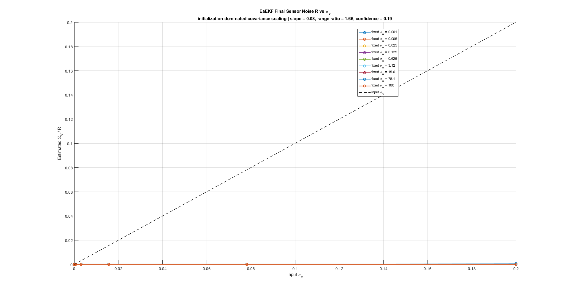
The EaEKF covariance diagnostic labels this run as initialization-dominated. Adaptation can be useful, but it does not erase the need to study initialization and excitation length.
Robustness evidence changes the estimator decision again. The current selection record combines nominal, covariance, initial-SOC, additive-noise, gain-bias, and Hall-bias studies. Under that weighting, Em7SPKF is selected; EsSPKF is the balanced fallback; and the nominally strong EacrSPKF is retained as a reference rather than the bundle-wide default.
Answers to the practical questions
- Can Bayes improve a poor starting point? It can explore continuously and the historical
EaEKFresult beats the coarse grid. The promoted artifacts do not contain a clean manual-before/Bayes-after control, so this repository does not quantify improvement over expert manual tuning. - Can Bayes validate a reasonable tuning? Yes. Near agreement with an independent grid for
ESC-EKF,ESC-SPKF, andEsSPKFin the paired study supports the same practical region with fewer evaluations. - Is the best Bayes point globally optimal? No such claim is supported. Both the historical
EacrSPKFmiss and the broader P25 disagreement show why. - Can optimization compensate for estimator/model mismatch? Only within the chosen objective and data. It does not rescue consistently poor estimators or guarantee transfer to injected faults.
Recommended protocol
- Pin the model, dataset, estimator implementation, objective, bounds, seed, and evaluation budget.
- Run Bayesian optimization as a sample-efficient candidate search.
- Inspect the optimization history when retained; this repository does not currently promote a tracked history plot for the P25 run.
- Validate the candidate with a local neighborhood or independent grid.
- Report best, mean, and worst behavior across covariance and initial-SOC sweeps—not only the minimum.
- Test explicit sensor corruptions before making a deployment decision.
- Promote the configuration and concise evidence together.
Reproducibility map
Bottom line
Bayesian optimization is valuable here because it makes a costly tuning search repeatable and can recover useful regions with fewer evaluations than a broad grid. Its scientific role is candidate generation plus empirical validation. Confidence comes from independent sweeps and robustness studies, not from the optimizer’s “best” label alone.